|
mlpack
blog
|
Quantum Gaussian Mixture Models - Week 3
In the week 2, I did calculate the integral of probabilities of QGMM, and the results is one from negative infinity to positive infinity.
This week, I'm curious what is the 2D shape of QGMM that I used for integral calculation, so I did draw the shape using matplotlib library in Python.
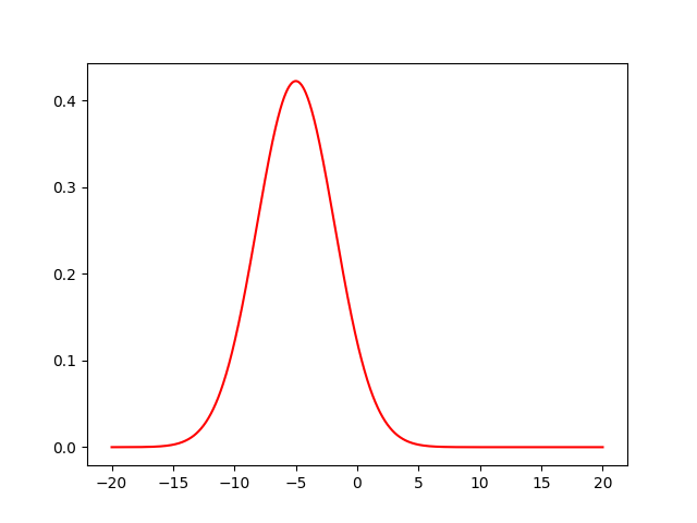
I used the two quantum Gaussian distributions, G1 and G2.
- G1 = [ mean: -5, covariance: 5 ]
- G2 = [ mean: 5, covariance: 5 ]
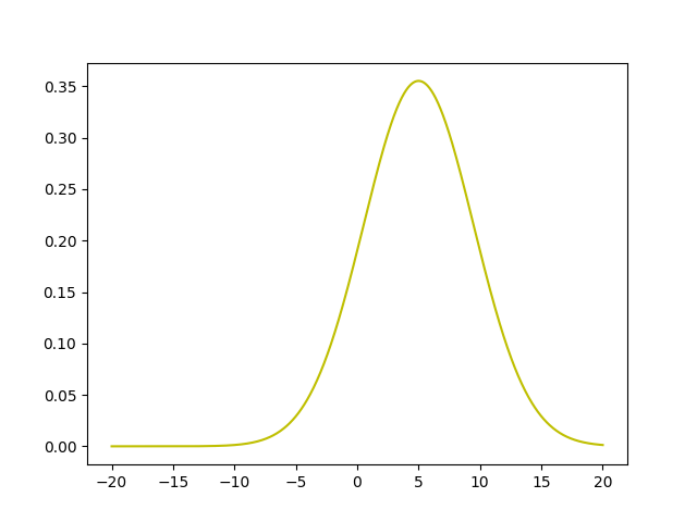
Below are the shape of each quantum Gaussian distribution.
[G2]
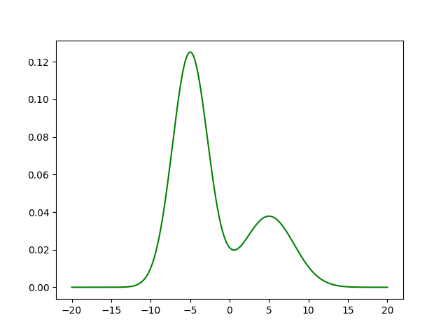
And below is the mixture of the two quantum Gaussian distributions when the weights of G1 and G2 are 0.7 and 0.3 respectively.
- Note
- Source codes: https://github.com/KimSangYeon-DGU/GSoC-2019/blob/master/Research/Code/qgmm_2d_plot.py
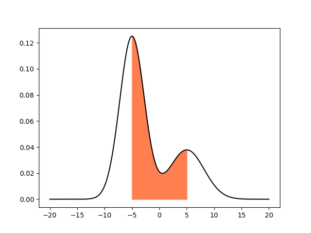
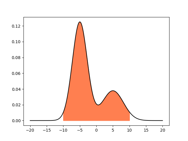
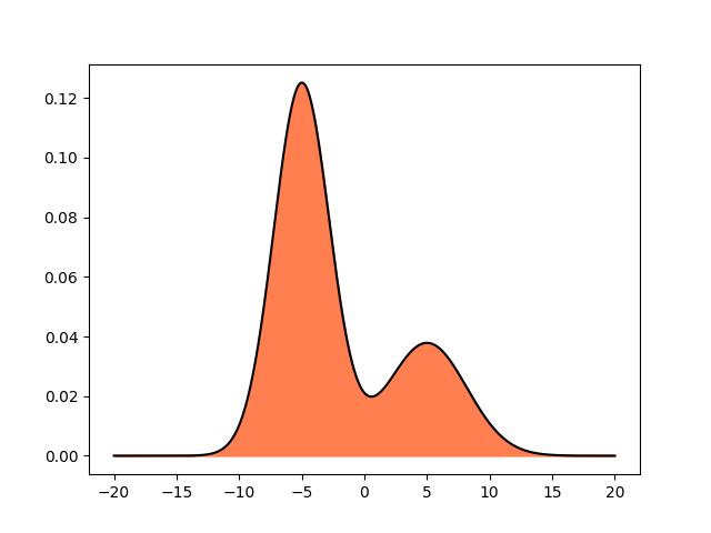
I also visualized the 2D integral area.
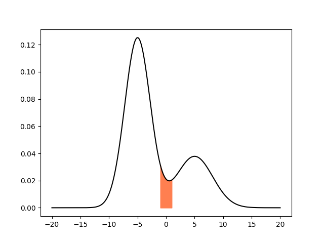
mean: 0, covariance: 5, probability: 0.4988
mean: 0, covariance: 10, probability: 0.974
mean: 0, covariance: 20, probability: 0.99
Through the meeting with the mentor, I decided the next step of our research is to check the validation of quantum EM algorithm using python code.
Next week, I'll check the validation of quantum EM algorithm.
Thanks for reading :)
Generated by
 1.8.13